In this post, we will improve our original optimization of the Johnson-Cook (J-C) material model parameters by considering the adiabatic heating of the material.

Why bother?
Firstly, there are materials with true stress-true strain dependencies that the J-C material model cannot describe adequately. Some materials exhibit a peak in the true stress-true strain dependency for specific strain rate and temperature ranges, followed by decreasing stress values at larger strains. However, when we look at the J-C model equation, we notice that it only allows stress to increase monotonically with strain at a constant strain rate and temperature. Usually, when we fit experimental curves to a material model, isothermal conditions are assumed. In the case of using the J-C model, we can’t model decreasing stress-strain behavior, and a numerical simulation with such model input may yield erroneous results.
Secondly, there’s the possibility of getting a better fit and reducing MAPE even for materials without a peak in the stress-strain curve.
Without going into details, let’s mention that the stress-strain curve is an interplay (principally) between strain and strain rate hardening on one side and dynamic softening mechanisms on the other. Strain rate and temperature determine which of the two will prevail.
Dynamic softening can lead to localization, which describes a concentration of plastic strain in specific material regions undergoing deformation. Localization can cause significant differences in material microstructure during hot forming processes, reducing material quality. So, appropriately describing this process is vital in FEM simulations of hot deformation processes.
What does the upgrade look like?
Adiabatic heating is pronounced in rapidly deformed materials. According to Johnson’s estimates, aluminum will heat adiabatically at strain rates approximately above 100 s⁻¹.
The model we will use is described by Smerd et al. and is given by the following equation:
ΔT is the specimen’s temperature increase, cp is specific heat, ρ density, σ stress, εp plastic strain, and β fraction of total plastic work converted into heat. The integral sums plastic work contributions at every strain increment. cp and ρ were assumed constant. The equation estimates the material’s temperature according to current strain and stress-strain curve behavior.
Until now in optimization, when we evaluated objective function values for a combination of parameters, the temperature was assumed constant. Now we presume temperature to be changing according to the upper rule.
β could be among the optimization parameters, but I decided first to test if the described update improves our solutions at all.
Does the adiabatic upgrade always work? 6061-T6 aluminum alloy example
Comparing MAPE values of the upgraded (β=0.9) and original optimization, we get these values:
| optimization type | best MAPE (%) |
| original | 3.1 |
| adiabatic upgrade (β=0.9) | 3.8 |
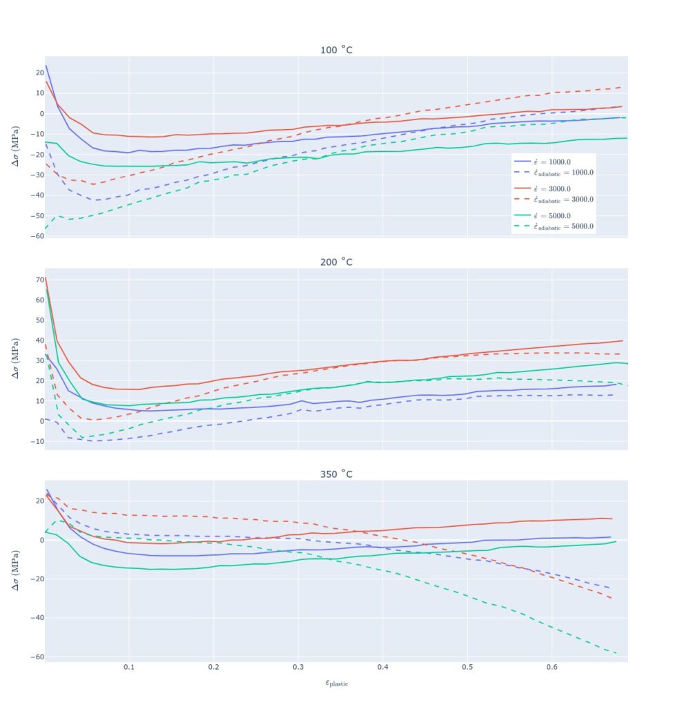
Wait, what? On average, the upgraded J-C was performing worse than the original solution. Differences between simulated (both original and upgraded) and experimental stress values are visualized below. With the adiabatic heating solution, the largest discrepancy from experimental values comes from high strain behavior at 350 °C and low strain behavior at 100 °C. Otherwise, fits produce very comparable results. The upgraded 200 °C example matches the original solution even better.

Lowering β resulted in gradually better results, and it seems like the adiabatic upgrade is unsuitable in this case. The adiabatic solution at 350 °C predicted decreasing stress values at higher strains, even though this was not observed experimentally.
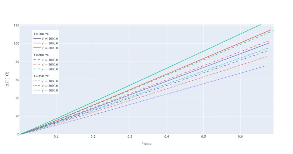
With β=0.9, temperature increases in a seemingly linear fashion. As expected, temperature rises the most with low temperatures and high strain rates.

Does the work at all? 7017-T6 aluminum alloy example
Because some of the high-temperature solutions from the previous section already displayed decreasing stress values after reaching a peak, I browsed through the literature in search of an aluminum alloy example with similar properties in the experimental stress-strain curve. I found it in a paper by Bobilli et al.
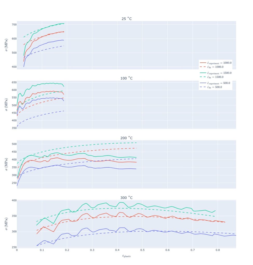
Stress-strain curves were digitized, but we can’t digitize what isn’t on the chart, though – some strain intervals are missing. Plastic strain onsets are already difficult to determine from crowded plots, even more so if the plastic strain onset region is not displayed. The highest temperature experiment reveals thermal softening. Such behavior is present in the adiabatic fit. This is a wonderful solution for me, although some other intervals are simulated poorly.

MAPE of the adiabatic solution is marginally better.
| optimization type | best MAPE (%) |
| original | 6.8 |
| adiabatic upgrade (β=0.9) | 6.5 |
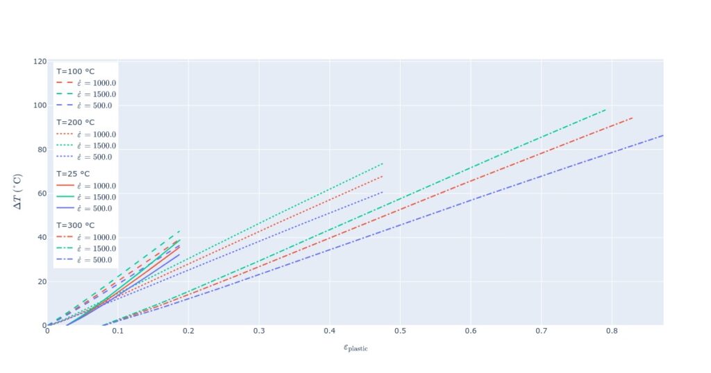
When we plot the estimated temperature increase of different samples, it is again a linear dependency. Its derivative is larger at lower temperatures. We can also notice a possible explanation for model underperformance – why does the 100 °C example predict a larger increase compared to 25 °C? As noted previously, the 25 °C case is missing stress-strain data for strains lower than 0.05, so according to our model, no temperature increase is assumed here because we cannot estimate it. Adiabatic upgrade considers erroneous temperatures at 25 and 300 °C.

Sidenotes
- We’re not discussing the engineering stress-strain dependency, where a similar peak and stress decrease are due to necking and assuming constant specimen cross-section.
- With data from Bobilli et al., different temperature examples cover different strain intervals. When the same number of points represented each stress-strain curve, MAPE of the original optimization was better than the adiabatic case, 7.6 % vs. 7.3 %. We obtain different results – see text body – if we weigh each curve differently while keeping the number of points per strain interval constant. A different number of points represents curves.
- Some authors use temperature-dependent specific heat and density. I kept these quantities constant because it seemed a needless complication compared to other simplifications.
- The adiabatic upgrade is a model, an assumption, not something realistic. Because recovery and recrystallization cause softening, it would be ideal to include something that can incorporate these processes, but it is not trivial.
Wrap-up
All in all, our upgrade is slightly better than the original if we compare MAPE only, but it can predict thermal softening, despite the issues with input data. Adiabatic upgrade inclusion makes sense if we deal with significant strain rates and if the material displays decreasing stress values at higher temperatures. Both of these properties are alloy dependent.
Some thermal softening may still occur in materials without decreasing stress values. Here, adiabatic optimization seemingly does not improve the result.
Material’s microstructure determines dynamic softening rates. To give a better description of the stress-strain curves, it would theoretically make sense to include microstructural parameters. In practice, estimating microstructural parameters is not straightforward, and there’s also the cost of doing many experiments to cover different conditions.
Lastly, let’s not forget true stress-true strain behavior can be decreasing even with (quasi)static strain rates. No adiabatic heating addition can circumvent this and is a material property that the J-C model cannot describe.
