Thought meanderings coupled with experiments in pursuit of filling own optimization knowledge gaps.

Motivation
The past year served me optimization problems more often than I feel comfortable admitting, and we’re not only talking about the casual hyperparameter tuning here. It stretched from optimizing prices for a car rental company to choosing optimal parameters for a numerical simulation of a metallurgical heating process, to name a few.
Although the problems have eventually been solved – albeit often not optimally, but outperforming manual search – many questions piled up along the way. In this blog, I try to tackle some of my blind spots and share some interesting insights. I’ll try to do so while confronting solutions from two Python optimization packages – Hyperopt and RBFOpt.
We’ll optimize on a mathematical formula to compare solutions with known optima and on a synthetic dataset to mock hyperparameter tuning in a machine learning problem.
Different kinds of optimization?
Something seemed off when considering how to put hyperparameter optimization and the usual mathematical optimization in the same post. Finding common points between the two optimization approaches was not straightforward, but are they really that different? Let’s try to shed some light on this question.
Understanding hyperparameter tuning is easy enough – we’re looking for a hyperparameter subset that results in the best (or, for our purpose, good enough) score. The score is whatever metric you choose; you only need to import it, like
from sklean.metrics import log_loss, mean_squared_error
The optimizer’s objective function output in this setting is the score of a machine learning model on validation data, and the goal of optimization is to find a hyperparameter subset that minimizes the score.
On the other hand, when you’re confronted with price optimization for a car rental company, there is some pain in deriving equations that calculate margin and consider whatever business logic you want to include. The goal of this type of optimization is, for example, to select such prices which optimize margin. The objective here is not an existing function; you must set it up manually.
Optimizing hyperparameters or prices does not sound that different anymore. How objective functions and constraints are set up sets apart business optimization problems from hyperparameter tuning.
What is a costly black box?
Hyperopt and RBFOpt are black-box optimizers, which means that the objective function formula is unknown, e.g., it could be a neural network score or a result of a numerical simulation. In other words, it can’t be evaluated with an equation.
If you can write your objective function down, such as a linear programming example with linear objective and constraints, you could omit using black-box optimizers and, for instance, the Python Pyomo library.
Both solvers are intended for examples where objective function evaluations are costly, meaning that objective evaluations take some time to compute and should use the least number of evaluations possible to reach a meaningful solution. Despite performing best for costly function evaluations, this does not mean you can not use them for examples where objective evaluations are rapid; it just means that, in this case, you are better off using a different method, such as a genetic algorithm.
Besides returning a machine learning model score or profit margin, the objective function could return many other things, and I invite you to be creative with your optimization use case. You could optimize distributions in a Monte-Carlo simulation, genetic operators in a genetic algorithm, or physical and material parameters in numerical simulations.
How do they work?
Black-box solvers can use existing objective function evaluations to construct an approximation of the objective function, often called a surrogate model. Note that it is not needed for a black-box optimizer to create a surrogate model. For example, genetic algorithms are black-box optimizers but don’t create a surrogate under the hood.
RBFOpt is deterministic, creating a surrogate using radial basis functions, and Hyperopt uses a probabilistic model – a type of Bayesian optimization – to approximate the objective function.
Both optimizers have in common that the surrogate model is used to select the next best step. At each iteration, an optimization is performed, and it is done on the current outlook of the surrogate itself. Of course, the minimum found is not necessarily the minimum of the original objective function, so the surrogate model is updated when new objective evaluations are available in the proposed coordinate. This process continues iteratively.
How will this post age?
The choice of Hyperopt and RBFOpt is arbitrary – I just happened to use these two recently. Still, their calculation approaches differ enough that it makes sense to investigate their convergence properties for different use cases. RBFOpt is deterministic and is typically not used to tune hyperparameters, but exploring how it performs in such a task seemed interesting.
Python package landscape is continuously evolving, so I’m not sure how well the content of this post will age. For the sake of being able to perform different kinds of optimizations, I included RBFOpt. Still, if hyperparameter tuning is your only goal, looking into scikit-optimize or hyperopt-sklearn makes more sense.
Optimization example of mathematical functions with known optima
To get a feel for how Hyperopt and RBFOpt perform, let’s first compare the calculated minimums of both solvers for two mathematical functions – sphere and Rastrigin function – which are often used as optimization benchmarks. In this case, the objective function is given as a mathematical expression, and the solution space is known and not stochastic.
Both examples are calculated with two parameters to easily visualize the comparison of estimated and known solutions. Search space is intentionally not zero-centered since RBFOpt adds the solution space geometric center to its initialized points.
Sphere function
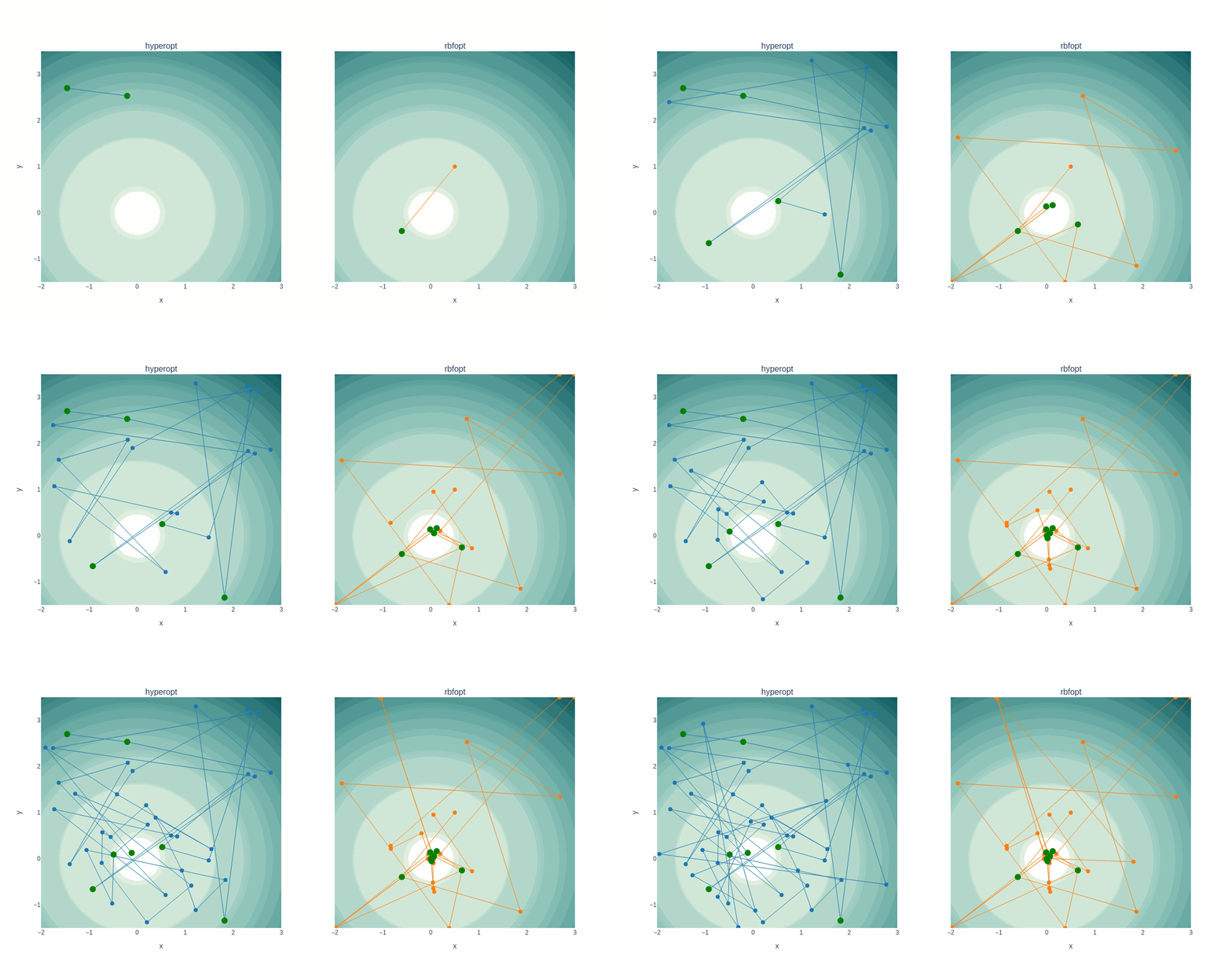
The animation below shows how both solvers select their next iteration. Each dot represents one step. A new best solution was found in the case of a green dot. One step is one iteration, so time flows differently for both plots. The contour plot shows the objective value.

The difference in traversing the search space for both solvers is evident and remarkable. We can see how Hyperopt chooses points spreaded along the entire search space, while RBFOpt concentrates points close to the existing best solution.

RBFOpt needed fewer iterations to reach a better solution. Regarding computation time, RBFOpt was slower to set up calculations. However, time comparisons here don’t make much sense because all computations were complete within fractions of a second.
RBFOpt’s convergence rate depends significantly on initial points; if a coordinate relatively close to the global minimum is included, it will need fewer iterations. There are a lot of parameters under the optimizer’s hood to control initial point selection (Latin hypercube, search space edges, etc.).
Rastrigin function
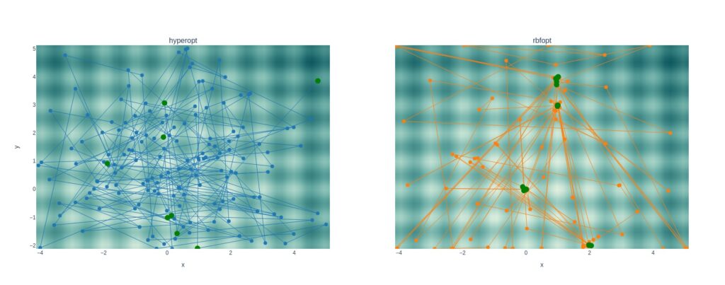
The same search space traversal properties as above are evident when tracing solutions to the Rastrigin function. The plot below displays the attempt and solution history after several iterations. Notice how RBFOpt concentrates points close to a solution found, and when it finds the next best solution, it hops there while making a couple of random jumps outside of these areas.
Also noteworthy is that Hyperopt could not pick up on the proper trough in the Rastrigin search space, whereas RBFOpt did. However, I don’t know if that is luck on the RBFOpt side.

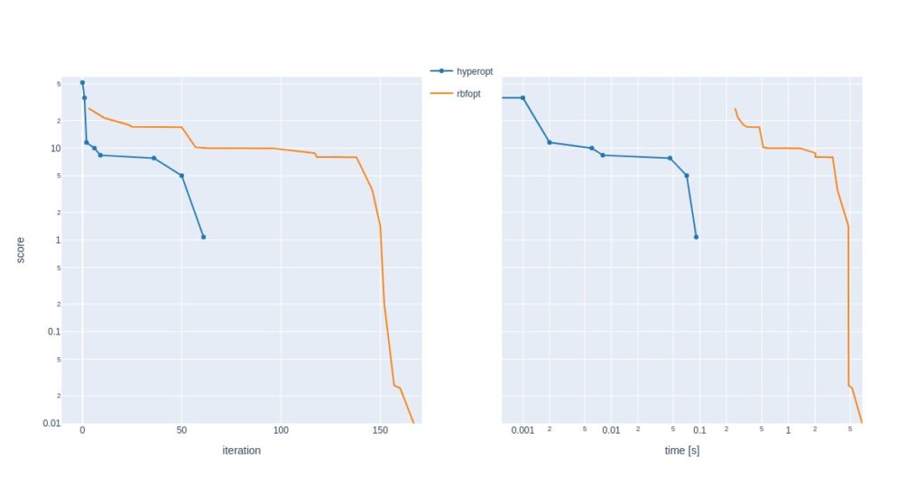
Not surprisingly, Hyperopt can find a decent solution much faster than RBFOpt. On the other hand, when RBFOpt iterates close enough to the global minimum, the calculated solution is much more accurate.

CatBoost model hyperparameter optimization
My experience with objective function properties in multidimensional hyperparameter search spaces is that they contain some randomness on an underlying smooth surface. You can often acquire comparable results with different hyperparameter settings, and obtaining a slightly better validation score does not always translate to a better test score.
In the following example, we used a CatBoost classifier, the metric was mean log loss of all validation sets in cross-validation, and we tuned only two hyperparameters, the number of iterations and learning rate. Other hyperparameters used default settings. It was a synthetic dataset.
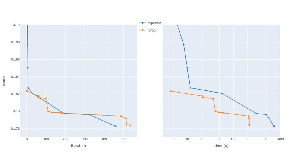
The required time to compute 1000 iterations was very different for both solvers; Hyperopt used 1512 seconds, and RBFOpt needed 365 seconds.
In 1000 runs, Hyperopt’s solution was best and achieved after slightly less than 500 steps. RBFOpt found the best one in a little over 500 steps. Hyperopt found its best solution in about 700 and RBFOpt in 200 seconds. I’d speculate that RBFOpt is faster than Hyperopt because of speedier estimations of the next best point.

Scores on test data paint the realistic picture of this analysis: the results are clearly overfitted, and our nitpicking did not result in any gains.
| method | best CV score | test score with best hyperparameters |
| grid search | 0.181 | 0.265 |
| RBFOpt | 0.178 | 0.273 |
| Hyperopt | 0.177 | 0.319 |
Technical notes
Some insights from along the way:
- Both optimizers were easy to set up.
- No attempts to optimize the optimizer’s parameters 🙂 have been made, although I’m confident one could do a lot, especially with RBFOpt and its massive number of settings. I never intended to go deep into it, but there may be much to discover.
- I enjoyed how easy it is to set up the search space in Hyperopt in case of discrete choices or different variable distributions (normal, lognormal, uniform). This can’t be done with RBFOpt.
- Hyperopt is generally faster, but expect a better solution with RBFOpt for non-stochastic objectives. Stochastic objective function solution improvements made with RBFOpt may not be relevant.
- Hyperopt traverses the search space more thoroughly.
- A great way to compare different machine learning model scores is by comparing Hyperopt trials. A bunch of calculations is made in the entire search space, which could include several machine learning algorithms. Later, we inspect results per algorithm and find those that perform better on our dataset.
- The findings above may not hold up against more dimensional examples.
- I would be very interested in investigating whether using Hyperopt and RBFOpt hand in hand may achieve better objective function values. The idea is that first, Hyperopt makes several calculations to approximately describe the search space, and secondly, RBFOpt uses the best solutions found to converge to an even better solution.
- When James Bergstra, Hyperopt co-creator, was asked how many iterations had been needed to find the minimum in his example with 238 parameters, he laughed and said he did not know. He used on the order of 1000 trials and added that “the purpose of Hyperopt is not always to completely optimize the space, it’s simply to do better than people.”
Wrap-up
This writing is a theoretical piece with experimental spice to find some inner peace regarding optimization. We discussed and played with Hyperopt and RBFOpt, and compared their solutions for mathematical equations and a synthetic dataset. Generally for more complex examples, it seems that Hyperopt will find a decent solution in less iterations and more time than RBFOpt. For peak precision in non-stochastic objectives, definitely give RBFOpt a try.
