An attempt to go beyond the usual standings table. This article is the analysis part of applying the PageRank algorithm to rank sports teams (coming soon).

What do we mean by ranking NBA teams? It is sorting them in order according to a metric used. A metric is a number that describes some aspect of a team’s quality, e.g., the total number of games won, average given points per game, or game pace. When we compare metrics of different teams, we can say which team is better and perhaps more likely to win. For example, a team with 10 winning games will likely lose against a team with 40 games won.
A typical ranking example is the usual standings table with win-loss percentages. We could enrich the standings table with info on teams’ averages. However, both winning percentages and stats based on past games still lack something I find crucial, and that is a team’s rank based on who it won or lost against and by how much.
Why win-loss percentages or past stats are not enough
NBA teams are divided into conferences and divisions. Each team plays its division rivals 4 times per season, other teams from the same conference 3 to 4 times, and opponents from the other conference 2 times each season. Divisions vary in strength, and similar could be said about both conferences.
Moreover, a game can be won or lost by chance. Or is it skill nonetheless? What do I know. 🙂
Both points above got me thinking that some teams may be biased in their win-loss percentages or other stats because they face either easier or more difficult opponents on average. In other words, their strengths of schedule vary. Or the ball didn’t go in in a tied match or went in more often than not. All that could also mean that a team’s standings position does not match its actual quality. The following analysis will try to shine some light on this issue. Google’s PageRank inspires the ranking algorithm used, and a discussion of my implementation is here (coming soon).
Teams’ performances vary during a season. For example, form, player injuries, and player trades all impact how a team performs. Usually, a standings table ranks teams based on all seasonal games. By just looking at the table, we have no idea if a team has recently been performing well or not and what was its strength of schedule. A ranking algorithm that gives more emphasis to recent games may overcome this issue. So let’s start by looking at a simple example of a time-dependent rank.
Team ranking example
Firstly, let’s look at the ranking results on team level. Time-dependent rank values are displayed in the plot below for Boston and Golden State, both NBA finalists in 2021/2022.
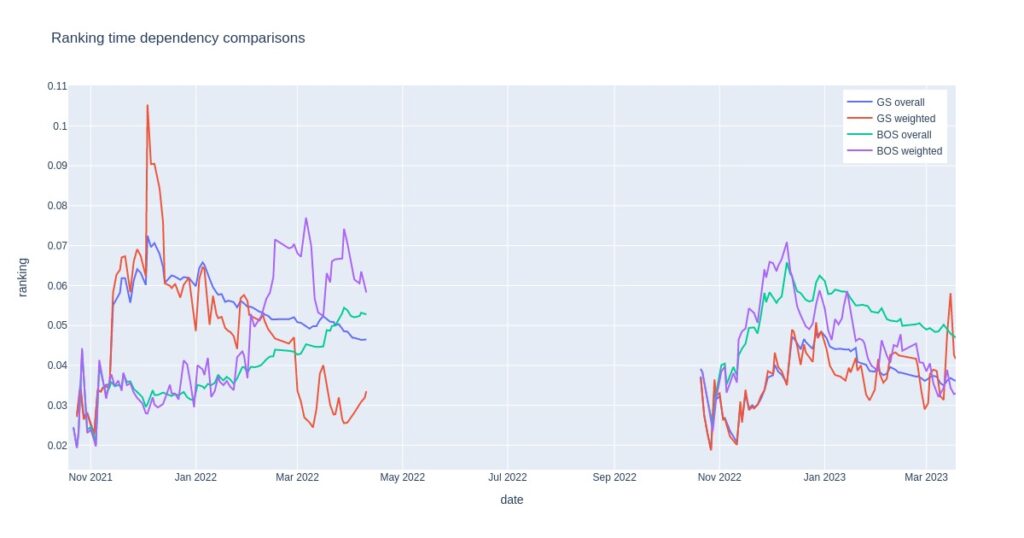
For each date, all games up to that date are included in ranking calculations, meaning the rank changes with time. Two curves represent each team: overall (all previous seasonal games included and given equal weight) and weighted (recent games are given more weight than past games).
Note that there are fewer games at the beginning of the season, making the overall calculation highly variable in this time interval. When games pile up during the season, overall ranking variability decreases, and values flatten out.
Overall rankings have less variability and show long-term team rank changes. Boston’s increasing form is particularly noticeable in the second part of 2021/2022, whereas Golden State’s rank decreased in the same period. On the other hand, Golden State seemed to dominate the first part of this season. In 2022/2023, Boston appears to be the better team among the two but is not displaying an increasing rank trend in the second part of the season so far.
Weighted values display variability that seems too large to be realistic but does not lag trends as much as the overall calculation.
Attention has yet to be put on optimizing parameters, which we will cover next.
Choosing the best damping factor
In research, a damping factor (sometimes also called randomization parameter) of 0.85 is often used when applying PageRank. Still, it would be worth looking into whether this setting is best for our example and how much it influences cumulative results.
The following plot looks at prediction accuracy and ROI as functions of damping factor.
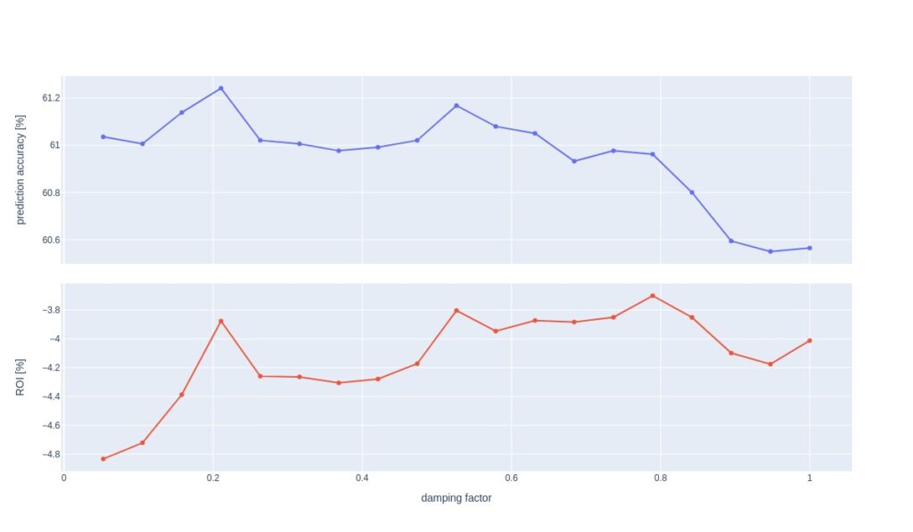
As we can see, prediction accuracy peaks at 0.2, corresponding to a local peak in ROI. However, because a lower optimal damping factor represents a higher degree of randomness and because neighboring points of 0.2 do not display similar behavior, I opt for 0.65 as optimum. This reasoning stems from eye inspection only, and we could go deeper into this also to try to understand the peak at 0.2.
We use 0.65 in all subsequent analyses, even for the weighted example. For the latter, the best damping factor may also be a function of the time constant.
Choosing the best smoothing factor and time constant for weighted rankings
Let’s repeat the process above to choose good smoothing factor and time constant parameters for weighted rankings. Since ranking time dependency curves display some jaggedness, exponentially weighted averaging is used to smooth it out; other approaches could freely be used.
First, adjacency matrix contributions are time-weighted. Later, this result is further smoothed. Different combinations of smoothing factor and time weight might produce similar results.
The contour plots below show how prediction accuracy and ROI depend on time constant and smoothing factor.
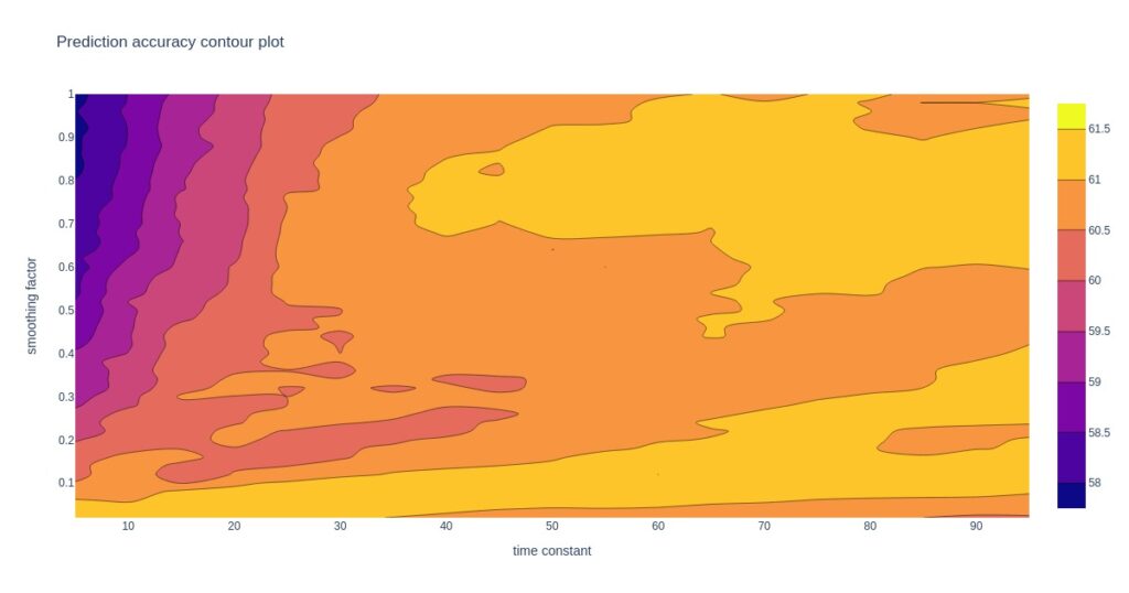
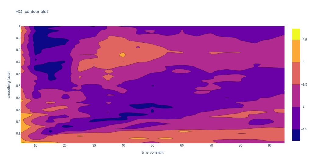
Looking at the contour plots, there may be more suitable regions for choosing a good pair of time constant and smoothing factor. All the following analysis uses a weighted ranking with a damping factor of 0.65, a smoothing factor of 0.75, and a time constant of 40. Some decent alternative options are at lower smoothing factors, but this exploration is left for another post.
The results of smoothing overall rankings are slightly worse than the one’s aboce and are not shown here.
After we have decided on the most suitable parameters, let’s explore the results.
Was it supposed to be a one-sided Boston game?
Dallas suffered a significant loss against Boston on January 5th, 2023, but according to past stats, the game should have been less one-sided. Of course, it might have been so if it wasn’t for Luka’s injury. The bookies, on the other hand, implied that Boston had a much greater probability of winning. Seeing all the hype and high expectations of Dallas (myself included) in Slovenia was interesting because of Luka’s brilliant recent performances.
It would be interesting to see the difference in rank values for these two teams. By no means do I expect it to give a clear favorite since it’s nearly impossible to fit all pre-game team knowledge in one feature, but let’s examine whether it tilts the scale more to Boston’s side.
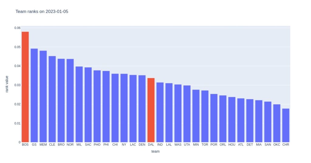
According to this feature, Boston was a clear favorite, but better rank does not always translate to success on the court. For example, Boston suffered a major loss to Oklahoma only a few nights before playing Dallas. Boston had at the time been ranked as number 1, whereas Oklahoma had been number 29, so our ranking approach is far from bullet-proof.
Oklahoma standings table vs. rankings
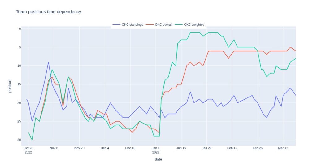
While we’re at Oklahoma, they have been a peculiar team this season. They started the season poorly but started gaining pace around surprisingly defeating Boston by a considerable difference. The chart below depicts this evolution in terms of positions on the standings table and ranking values. We can see that the table positioning started to improve, albeit slowly, after turning turbo on. Currently, they are a contender for the play-in.
Current position estimations
We end our analysis by comparing the standings table and weighted ranking positions for all teams. Note that positions are valid only on March 21st, 2023, and weighted rank positions display recent trends.
| Team | Standings table position | Weighted ranking position |
| MIL | 1 | 2 |
| BOS | 2 | 14 |
| PHI | 3 | 1 |
| DEN | 4 | 7 |
| CLE | 5 | 6 |
| MEM | 6 | 3 |
| SAC | 6 | 16 |
| NY | 8 | 10 |
| BRO | 9 | 19 |
| PHO | 10 | 4 |
| MIA | 11 | 18 |
| LAC | 12 | 12 |
| GS | 13 | 9 |
| ATL | 14 | 13 |
| DAL | 14 | 17 |
| MIN | 16 | 15 |
| TOR | 16 | 11 |
| OKC | 18 | 8 |
| LAL | 19 | 21 |
| UTA | 20 | 28 |
| NOR | 21 | 25 |
| CHI | 22 | 5 |
| IND | 23 | 23 |
| WAS | 23 | 22 |
| POR | 25 | 27 |
| ORL | 26 | 20 |
| CHR | 27 | 24 |
| HOU | 28 | 29 |
| SAN | 28 | 26 |
| DET | 30 | 30 |
Some teams I find particularly interesting in the table above are Oklahoma, Chicago, and Phoenix, with performances above expectations and underperforming Boston, Sacramento, and Brooklyn.
Wrap-up
In this article, we’ve seen how PageRank-influenced ranking can be used to rank NBA teams. The idea itself is not new. One thing I dislike about online prediction providers (free or paid) is that we cannot obtain past predictions, backtest them properly and see how they perform in practice, even though the content may indeed be splendid. To overcome this issue, I’ve developed my own ranking algorithm, even if the maths behind it isn’t PhD nor Stanford level.
The described flavor of ranking is a good approach to analyzing team performance, but it also comes with many cons and does not make predicting a single game any more straightforward than before. In my view, the main drawback of the current approach is that it does not include player information; Denver is not the same team if Jokić is missing, same for Dallas and Dončić, Milwaukee and Giannis, etc. However, the algorithm would enable tracking team performance changes after a notable trade or important player injury.
As with car trump cards from the top of the article, more rankings and other metrics should be used to give a more in-depth description of a team’s performance. Even though the article opened some new questions, let’s end it for today.
