Applying a genetic algorithm to find the best fit of a material model to experimental stress-strain curves for aluminum alloy 6061 in peak-aged condition.

Why I find it important
I started my career doing simulations for a metallurgical company. Misfits between experiments and simulations were a (stressful) regular occurence, and I spent a lot of (even more stressful) time manually searching parameter subsets that resulted in acceptable solutions.
Often solutions were not acceptable but were at least descriptive. For example, we could get a sense of what temperature or stress fields looked like during extrusion or casting. Still, it was not accurate enough to steer processes for new alloys or substantially improve existing process parameters, like maximizing casting speed.
To this day, not being able to achieve better simulation results still stings me a lot. At the time, I knew little about optimization, but I’ve meandered to the field in recent years, so imagine my surprise when someday a great idea popped up – fit simulations to experiments using optimization algorithms or optimize a process entirely.
This post is an excerpt of a service I’ve developed for my clients since: finding a suitable material model that speeds up development time, describes the simulated process better, and helps achieve better overall results.
Choice of material model
As the title already suggests, we will try to find the best material parameters of the Johnson-Cook (J-C) material model:
It is simple enough, widely used, and heavily supported in commercial FEM solvers. The model is empirical, meaning its parameters don’t represent physical quantities, such as the activation energy in the Zerilli-Armstrong model. On one side, we don’t have to poke through literature in search of suitable parameter intervals for our specific alloys. Secondly, we don’t need expensive or time-consuming experiments to extract quantities like dislocation cell sizes.
Another reason why J-C is a good candidate for tuning parameters using optimization is because some of the existing calibration approaches don’t necessarily find good solutions, or parameter calculation is simplified. Shortcuts have their merits but can leave some parameter subspaces poorly described.
I’ll fit the J-C model to experimental data using Hyperopt and a genetic algorithm (GA).
Data preparation
I used experimental data from a paper by Lee and Tang. The authors assessed stress-strain curves at different strain rates (0.001, 1000, 3000, 5000 s⁻¹) and temperatures (100, 200, 350 ˚C), perfect for our use case.
Stress-strain curves were digitized with WebPlotDigitizer. Especially when many curves are plotted closely to one another at small intervals, it is difficult not to make errors digitizing data. Preparing good quality stress-strain curve data – either by creating own experiments or digitization – is crucial for obtaining the best possible results, so preprocessing pays off.
Curves were digitized, plastic strain onsets were determined, and only plastic deformation data were used; equidistant strain points were calculated, and interpolated stress values were evaluated at these points.
Metric selection
In traditional machine learning, you’d leave out a test dataset to check the validity of your model on unseen data. Here, the experiments are so scarce you use everything you have to obtain the best fit and compare the fit to the model, which I did too.
Curves for all strain rates and temperatures were evaluated at equidistant points, and the number of points for all curves was the same. In doing so, all curves had the same weights, and all curve intervals were weighted the same.
From my experience, when researchers calculate material parameters through optimization, the metric they use is mostly MSE. For some aluminum series 6000 alloys (also depending on the temper), stress can increase from 150 MPa (yield stress) to 250 MPa (tensile strength). A model error of 30 MPa is around 20 % at low and 10 % at higher strains, a considerable difference that MSE can’t account for. To get around this issue, I decided to use MAPE.
Results
Optimization parameters were A, B, C, n, m, ε’₀. Reference and melting temperatures were kept constant. When fitting the material model, all experimental curves were used except the one with a strain rate of 0.001 s⁻¹.
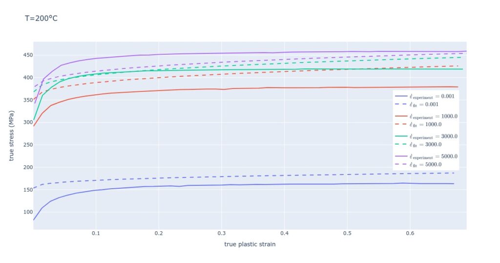
After several tests, Hyperopt struggled with convergence to global minima when search space intervals were too wide, whereas GA did not have these issues. GA was the faster solver since it reached the same quality solution faster, and its minimum MAPE was lower than Hyperopt’s.
| optimization algorithm | best MAPE (%) | required time (s) |
| Hyperopt | 3.9 | 245 |
| GA | 3.1 | 39 |
For these reasons, GA optimal solution is used in subsequent analyses with the following parameters:
| A (MPa) | B (MPa) | n | C | m | ε’₀ (s⁻¹) |
| 416 | 152 | 0.18 | 0.10 | 2.29 | 13537 |
The downside of GA is getting slightly different results each time if the random seed is not fixed and not knowing if the obtained result is a global optimum.
First, let’s look at the comparison between experimental and simulated data. The simulated stress-strain curve is concave and follows the experimental curve decently; some Hyperopt solutions were local optima because simulated stress-strain curves were convex.

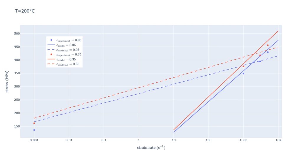
When discussing results with my clients, I show them what the model predicts for strain rates/temperatures/strains not covered by experiments. The plot below shows one such example. Interestingly, when Lee and Tang build their constitutive model, the 0.001 strain rate example is omitted, and from the plot below it is quickly clear why. Extrapolating the model prediction to lower strain rates results in huge errors at lower strain rates, despite capturing high strain rate dependence well. On the other hand, if the 0.001 strain rate curve is included in the calculation, the fit is poor overall but can be used throughout the strain rate interval.

The last plot shows how a model (under)performs when the 0.001 curve is included in the calculation.

Sidenotes
- Ideally, we want to feed true stress-true strain behavior to the material model. Sometimes this data is unavailable, so we can use the engineering relationships on a narrower strain interval instead.
- When a decent solution is found, we should keep in mind that it does probably not generalize well to other tempers, slightly different chemical compositions, and different processing conditions, for example, extrusion temperatures or post-homogenization cooling rates.
- We could tweak the optimizers’ hyperparameters to get a better solution. However, the contribution of tweaking fades compared to considering actual specimen temperatures. Due to large strain rates, heating is adiabatic and not isothermal. The next step would include actual specimen temperature, even if only approximate.
- Defining search space properties – distribution type and range – speeds up both solvers considerably. Including domain knowledge on expected parameter ranges can help a lot.
- One explanation for why including 0.001 strain rate data results in bad fits is that it was obtained using a different experiment.
- When performing these types of analyses for my clients, I’d usually ask them to estimate ranges of strains, strain rates, and temperatures in their process. Knowing these properties, I can tailor the metric to best describe their intervals of interest by giving more weight to these regions in MAPE calculations, for example.
- Customizing the solver’s objective function makes using different metrics or applying unequal weights to curves or strain intervals easy.
Conclusion
Overall, we showed how to use optimization algorithms to speed up the calculation of adequate material parameters, which simulation engineers can readily include in their FEM simulations, achieving better results and shortening the development cycle.
